Training Modes
SuperGradients allows users to train models on different modes: 1. CPU 2. single GPU - (CUDA) 3. multiple GPUs' - Data Parallel (DP) 4. multiple GPUs' - Distributed Data Parallel (DDP)
1. CPU
Requirement: None.
How to use it: If you don't have any CUDA device available, your training will automatically be run on CPU.
Otherwise, the default device will be CUDA, but you can still easily set it to CPU using setup_device as follow:
from super_gradients import Trainer
from super_gradients.training.utils.distributed_training_utils import setup_device

setup_device(device='cpu')

# Unchanged
trainer = Trainer(...)
trainer.train(...)
2. CUDA
Requirement: Having at least one CUDA device available
How to use it: If you have at least one CUDA device, nothing! Otherwise, you will have to use CPU...
3. DP - Data Parallel
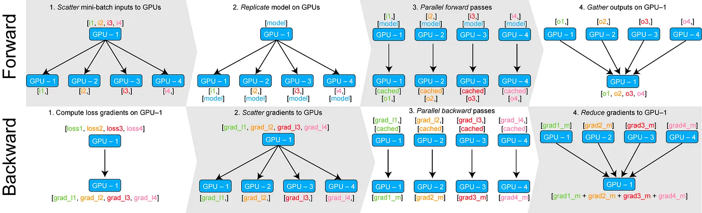
DataParallel (DP) is a single-process, multi-thread technic for scaling deep learning model training across multiple GPUs on a single machine.
The general flow is as below
- Split the data into smaller chunks (mini-batch) on GPU:0
- Move one chunk of data per GPU
- Copy the model to all available GPUs
- Perform the forward pass on each GPU in parallel
- Gather the outputs on GPU:0
- Compute the loss on GPU:0
- Share the loss to all the GPUs
- Compute the gradients on each GPU
- Gather and sum up gradients on GPU:0
- Update model on GPU:0
For more detailed information, feel free to check out this blog for a more in-depth explanation.
Requirement: Having at least one CUDA devices available
How to use it: All you need to do is to call a magic function setup_device before instantiating the Trainer.
from super_gradients import Trainer
from super_gradients.training.utils.distributed_training_utils import setup_device

# Launch DP on 4 GPUs'
setup_device(multi_gpu='DP', num_gpus=4)

# Unchanged
trainer = Trainer(...)
trainer.train(...)
setup_device as early as possible.
4. DDP - Distributed Data Parallel
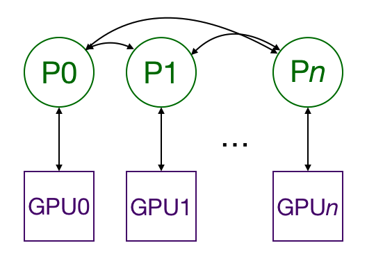
Distributed Data Parallel (DDP) is a powerful technique for scaling deep learning model training across multiple GPUs. It involves the use of multiple processes, each running on a different GPU and having its own instance of the model. The processes communicate only to exchange gradients, making it a highly efficient and more scalable solution for training large models than Data Parallel (DP).
Although DDP can be more complex to set up than DP, the SuperGradients library abstracts away the complexity by handling the setup process behind the scenes. This makes it easy for users to take advantage of the benefits of DDP without having to worry about technical details. We highly recommend using DDP over DP whenever possible.
For more detailed information, feel free to check out this blog for a more in-depth explanation.
Requirement: Having multiple CUDA devices available
How to use it: All you need to do is to call a magic function setup_device before instantiating the Trainer.
from super_gradients import Trainer
from super_gradients.training.utils.distributed_training_utils import setup_device

# Launch DDP on 4 GPUs'
setup_device(num_gpus=4) # Equivalent to: setup_device(multi_gpu='DDP', num_gpus=4)

# Unchanged
trainer = Trainer(...)
trainer.train(...)
setup_device as early as possible.
What should you be aware of when using DDP ?
A. DDP runs multiple processes
When running DDP, you will work with multiple processes that will go through the whole training loop. This means that if you run DDP on 4 gpus, any action that you do will be run 4 times.
This impacts especially printing, logging, and file writing. To face this issue, SuperGradients provides a decorator that will ensure that only one process will execute a specific function, whether you work with CPU, GPU, DP, or DDP.
In the following example, the print_hello function will print Hello world only once, when it would be printed 4 times without the decorator...
from super_gradients.training.utils.distributed_training_utils import setup_device
from super_gradients.common.environment.ddp_utils import multi_process_safe

setup_device(num_gpus=4)

@multi_process_safe # Try with and without this decorator
def print_hello():
    print('Hello world')

print_hello()
B. DDP requires specific Metric implementation!
As explained, multiple processes are used to train a model with DDP, each on its own GPU. This means that the metrics must be computed and aggregated across all the processes, and it requires the metric to be implemented using states.
States are attributes to be reduced. They are defined using the built-in method add_state() and enable broadcasting
of the states among the different ranks when calling the compute() method.
An example of a state would be the number of correct predictions, which will be summed across the different processes, and broadcasted to all of them before computing the metric value. You can see an example below.
Feel free to check torchmetrics documentation for more information on how to implement your own metric.
Example In the following example, we start with a custom metric implemented to run on a single device:
import torch
from torchmetrics import Metric


class Top5Accuracy(Metric):
    def __init__(self):
        super().__init__()
        self.correct = torch.tensor(0.)
        self.total = torch.tensor(0.)

    def update(self, preds: torch.Tensor, target: torch.Tensor):
        batch_size = target.size(0)

        # Get the top k predictions
        _, pred = preds.topk(5, 1, True, True)
        pred = pred.t()

        # Count the number of correct predictions only for the highest 5
        correct = pred.eq(target.view(1, -1).expand_as(pred))
        correct5 = correct[:5].reshape(-1).float().sum(0)

        self.correct += correct5.cpu()
        self.total += batch_size

    def compute(self):
        return self.correct.float() / self.total
self.correct and self.total with add_state and to define
a reduce function dist_reduce_fx that will be used to know how to combine the states when calling compute:
import torch
import torchmetrics

class DDPTop1Accuracy(torchmetrics.Metric):
    def __init__(self, dist_sync_on_step=False):
        super().__init__(dist_sync_on_step=dist_sync_on_step)

        self.add_state("correct", default=torch.tensor(0.), dist_reduce_fx="sum")   # Set correct to be a state
        self.add_state("total", default=torch.tensor(0), dist_reduce_fx="sum")      # Set total to be a state

    def update(self, preds: torch.Tensor, target: torch.Tensor):
        batch_size = target.size(0)

        # Get the top k predictions
        _, pred = preds.topk(5, 1, True, True)
        pred = pred.t()

        # Count the number of correct predictions only for the highest 5
        correct = pred.eq(target.view(1, -1).expand_as(pred))
        correct5 = correct[:5].reshape(-1).float().sum(0)

        self.correct += correct5
        self.total += batch_size

    def compute(self):
        return self.correct.float() / self.total
update() method modifies the internal state of each instance in each process based on the inputs preds and target specific to that process.
3. After an epoch, each process will have a unique state, for example:
- Process 1: correct=50, total=100
- Process 2: correct=30, total=100
- Process 3: correct=100, total=100
4. Calling compute() triggers torchmetrics.Metric to gather and combine the states of each process. This reduction step can be customized by setting the dist_reduce_fx, which in this case is the sum. This usually happens at the end of the epoch.
- All processes: correct=180, total=300
5. The compute() method then calculates the metric value according to your implementation. In this example, every process will return the same result: 0.6 (180 correct predictions out of 300 total predictions).
6. Finally, calling reset() will reset the internal state of the metric, making it ready to accumulate new data at the start of the next epoch.
C. When using DDP you may want to scale the learning rate
Using N GPUs in DDP mode, has an effect of increasing batch size by a factor of N. And it has been shown that it may be necessary to scale the learning rate accordingly. The rule of thumb is that if batch size is increased by a factor of N (Or N nodes used in DDP), the learning rate should be also increased by a factor of N.
However, when it comes to adaptive optimizers like Adam, the situation is a bit different. Adaptive optimizers like Adam automatically adjust the learning rate for each parameter based on the historical gradient information. They inherently adapt to the scale of the gradients and don't require manual adjustments of the learning rate in the same way as fixed learning rate methods like SGD.
That being said, we still recommend to try out different learning rates to see the impact on the final metrics. You can run experiments manually or use Hydra sweep syntax to run experiments with custom learning rates as follows:
python -m super_gradients.train_from_recipe -m --config-name=coco2017_yolo_nas_s training_hyperparams.initial_lr=1e-3,5e-3,1e-4
How to set training mode with recipes ?
When using recipes you simply need to set values of gpu_mode and num_gpus.
# training_recipe.yaml
default:
   - ...

...

# Simply add this to run DDP on 4 nodes.
gpu_mode: DDP
num_gpus: 4