Training an external model
In this example we will use SuperGradients to train a deep learning segmentation model to extract human portraits from images, i.e., to remove the background from the image.
We will show how SuperGradients allows seamless integration of an external model, dataset, loss function, and metric into the training pipeline.
Quick installation
For this example, the only necessary package is super-gradients. Installing super-gradients will also install all dependencies required to run the code in this example.
pip install super-gradients
1. Dataset
The dataset we will use in this example is the AISegment dataset, available to download for free from Kaggle. The dataset contains 34,427 RGB images of human portraits and their corresponding soft masks. The provided images are center-cropped to a unified shape of 600x800.
1.A. Data preparation
The original structure of the data on the disk is as follows:
data
└───aisegment-matting
│   └───matting
│       │   └───1803290511
│       │   │       └───matting_00000000
│       │   │       │         1803290511-00000459.png
│       │   │       │         1803290511-00000458.png
│       │   │       │         ..
│       │   └───1803290444
│       │       ..
│   └───clip_img
│       │   └───1803290511
│       │   │       └───clip_00000000
│       │   │       │         1803290511-00000459.jpg
│       │   │       │         1803290511-00000458.jpg
│       │   │       │         ..
│       │   └───1803290444
│       │       ..
In the structure shown above, the clip_img directory contains the portrait images, divided into many
sub-directories. The matting directory is structured similar to the clip_img directory, containing
the corresponding masks. This structure is not particularly convenient for data loading, therefore
we will first rearrange the data with the following script, which only requires changing the data_path and
out_path variables:
import random
import shutil
from pathlib import Path


data_path = Path('/path/to/original/data/directory')
out_path = Path('/path/to/output/data/directory')

# Create output directories
out_path.mkdir(exist_ok=True)

train_out_path = out_path / "train"
val_out_path = out_path / "val"
test_out_path = out_path / "test"

train_out_path.mkdir(exist_ok=True)
val_out_path.mkdir(exist_ok=True)
test_out_path.mkdir(exist_ok=True)

# Get all image and mask path
all_image_paths = data_path.rglob('*.jpg')
all_mask_paths = data_path.rglob('*.png')

# Map filenames (without extensions) to image paths
filename_map = {}
for img_path in all_image_paths:
    filename_map[img_path.stem] = img_path

# Get all matching image-mask path pairs
path_pairs = []
for mask_path in all_mask_paths:
    filename = mask_path.stem
    if filename in filename_map:
        path_pairs.append((filename_map[filename], mask_path))
        del filename_map[filename]

# Split to train, validation, and test sets
random.seed(1)
val_samples = random.sample(path_pairs, k=int(0.1*len(path_pairs)))
test_samples = random.sample(list(set(path_pairs)-set(val_samples)), k=int(0.1*len(path_pairs)))
train_samples = list(set(path_pairs)-set(val_samples)-set(test_samples))

# Copy data to new location
for img_path, mask_path in train_samples:
    shutil.copy(img_path, train_out_path)
    shutil.copy(mask_path, train_out_path)

for img_path, mask_path in val_samples:
    shutil.copy(img_path, val_out_path)
    shutil.copy(mask_path, val_out_path)

for img_path, mask_path in test_samples:
    shutil.copy(img_path, test_out_path)
    shutil.copy(mask_path, test_out_path)
The original data may have images without their corresponding masks. Therefore, the above code first finds all existing image-mask pairs. It then splits the data into train/validation/test sets, where the size of each of the validation and test sets is 10% of the total number of samples. The samples in each of the sets are then copied to the output path, structured as follows:
data
    └───train
    │       1803290511-00000029.jpg
    │       1803290511-00000029.png
    │       ..
    └───val
    │       1803290444-00000292.jpg
    │       1803290444-00000292.png
    │       ..
    └───test
    │       1803290443-00000294.jpg
    │       1803290443-00000294.png
    │       ..
Each of the train/val/test directories contain all image (.jpg) files and their corresponding mask (.png) files.
1.B. PyTorch Dataset
In some cases, we may want to have full control over the process of loading and pre-processing the training data. SuperGradients is fully compatible with PyTorch data loaders, which allows for seamless integration of custom dataset implementations for maximum flexibility.
We will first present the complete Dataset class implementation, and then break it down to fully understand what is going on.
import os
from PIL import Image
import torch
from torchvision.transforms import transforms as torch_transforms
from super_gradients.training.transforms.transforms import SegColorJitter, SegRandomFlip, SegResize


class AISegmentDataset(torch.utils.data.Dataset):
    NORMALIZATION_MEANS = [.485, .456, .406]
    NORMALIZATION_STDS = [.229, .224, .225]

    def __init__(self, data_path: str, split: str, input_height: int = 256, input_width: int = 256):
        if split not in ['train', 'val', 'test']:
            raise ValueError("The 'split' parameter must be either 'train', 'val', or 'test'")

        self.split = split
        self.input_height = input_height
        self.input_width = input_width

        data_path = os.path.join(data_path, split)

        self.path_pairs = []
        for filename in os.listdir(data_path):
            if filename.endswith('.jpg'):
                self.path_pairs.append((os.path.join(data_path, filename),
                                        os.path.join(data_path, filename.replace('.jpg', '.png'))))

    def __len__(self):
        return len(self.path_pairs)

    def __getitem__(self, idx):

        image = Image.open(self.path_pairs[idx][0]).convert('RGB')
        mask = Image.open(self.path_pairs[idx][1]).split()[-1]

        if self.split == 'train':
            seg_transforms = torch_transforms.Compose([
                SegRandomFlip(prob=0.5),
                SegColorJitter(brightness=0.5, contrast=0.5, saturation=0.5),
                SegResize(h=self.input_height, w=self.input_width)
            ])
        else:
            seg_transforms = SegResize(h=self.input_height, w=self.input_width)

        transformed_pair = seg_transforms({"image": image, "mask": mask})
        image, mask = transformed_pair['image'], transformed_pair['mask']

        image_transform = torch_transforms.Compose([
            torch_transforms.ToTensor(),
            torch_transforms.Normalize(self.NORMALIZATION_MEANS, self.NORMALIZATION_STDS)
        ])
        mask_transform = torch_transforms.ToTensor()

        image_tensor, mask_tensor = image_transform(image), mask_transform(mask)

        return image_tensor, mask_tensor
First, we can see that our dataset class inherits from the torch.utils.data.Dataset class. To initialize the dataset
object, two parameters must be provided:
data_path- the full path to the data's root directorysplit- a string indicating whether this is the 'train', 'val', or 'test' split of the data
Additional parameters include input_height and input_width, the fixed height and width, respectively, for resizing
the input images and masks. These are set to 256 by default. At the end of the initialization function, the image and
mask path pairs are determined according to the split.
Next, let's see what happens when we retrieve an item from the dataset via the __getitem__() function.
First, an image and its corresponding mask are loaded according to the idx parameter:
image = Image.open(self.path_pairs[idx][0]).convert('RGB')
mask = Image.open(self.path_pairs[idx][1]).split()[-1]
Notice that we take only the mask's last channel. The mask's original color format is RGBA, and the alpha channel should be used as the soft mask for segmentation according to the dataset's description.
Next, we apply transformations to the image and mask according to the split:
if self.split == 'train':
    seg_transforms = torch_transforms.Compose([
        SegRandomFlip(prob=0.5),
        SegColorJitter(brightness=0.5, contrast=0.5, saturation=0.5),
        SegResize(h=self.input_height, w=self.input_width)
    ])
else:
    seg_transforms = SegResize(h=self.input_height, w=self.input_width)

transformed_pair = seg_transforms({"image": image, "mask": mask})
image, mask = transformed_pair['image'], transformed_pair['mask']
On training images and masks we apply data augmentation: a random horizontal flip with probability 0.5, and
random color jitter which randomly changes the image's brightness, contrast, and saturation. Both the training and the
other splits' images and masks undergo resizing according to input_height and input_width.
The transforms in the above code are all SuperGradients transforms, which are built upon PyTorch's
torchvision.transforms. This allows for maximum compatibility with PyTorch components. For example, we can see that
the transforms are sequentially composed using torchvision's Compose class. Notice also that the transform names are
all prefixed with Seg - meaning that they are specifically designed for segmentation data. These transforms take care
to apply the same transformation to the image and the mask when required, or only apply the transformation to the image
otherwise. For example, if SegRandomFlip() flips the image, the mask will be flipped as well. SegColorJitter() only
transforms the image. SegResize() resizes both the image and the mask.
Next, we convert the image and the mask to PyTorch Tensors, and normalize the image using the NORMALIZATION_MEANS and
NORMALIZATION_STDS:
image_transform = torch_transforms.Compose([
    torch_transforms.ToTensor(),
    torch_transforms.Normalize(self.NORMALIZATION_MEANS, self.NORMALIZATION_STDS)
])
mask_transform = torch_transforms.ToTensor()

image_tensor, mask_tensor = image_transform(image), mask_transform(mask)
These transforms are applied regardless of the current dataset split. Notice that here we use torchvision transforms. This serves to show the high degree of flexibility SuperGradients allows, as its transforms are based on PyTorch's torchvision transforms which may be used interchangeably.
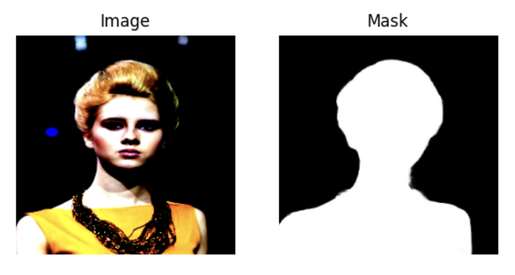
1.C. Data visualization
To conclude this section, let's visualize some images and their masks to test our AISegmentDataset implementation. First, we instantiate two dataset objects, for the training and validation splits, and extract the first sample from each:
import matplotlib.pyplot as plt

data_path = '/path/to/arranged/data/dir'

train_dataset = AISegmentDataset(data_path=data_path, split='train')
val_dataset = AISegmentDataset(data_path=data_path, split='val')

train_image, train_mask = train_dataset[0]
val_image, val_mask = val_dataset[0]
Let's first visualize the validation image and mask:
figure = plt.figure()
figure.add_subplot(1, 2, 1)
plt.title("Image")
plt.axis("off")
plt.imshow(val_image.permute(1, 2, 0))
figure.add_subplot(1, 2, 2)
plt.title("Mask")
plt.axis("off")
plt.imshow(val_mask.squeeze(), cmap='gray')

plt.show()
And the training image and mask:
figure = plt.figure()
figure.add_subplot(1, 2, 1)
plt.title("Image")
plt.axis("off")
plt.imshow(train_image.permute(1, 2, 0))
figure.add_subplot(1, 2, 2)
plt.title("Mask")
plt.axis("off")
plt.imshow(train_mask.squeeze(), cmap='gray')

plt.show()
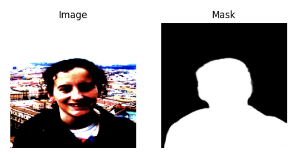
We can see the effect of the color jitter transform on the image.
2. Model architecture
For this example we will employ the U-Net architecture. U-Net and its variants are a popular choice for many image segmentation tasks. It is a fully-convolutional architecture, consisting of an expanding and a contracting path with skip connections between the encoder and decoder blocks. In this example we will demonstrate how we can easily integrate an external PyTorch model as part of SuperGradients' training pipeline. To this end, we will use a U-Net implementation loaded directly from PyTorch Hub:
model = torch.hub.load('mateuszbuda/brain-segmentation-pytorch', 'unet', in_channels=3, out_channels=1,
                       init_features=32, pretrained=False)
Since our model's inputs are RGB images, we set in_channels=3. This is a binary segmentation task, therefore
out_channels=1. The init_features parameter determines the number of kernels in the first block's convolution
layers. The number of kernels is doubled in each consecutive encoder block. We also set pretrained=False since
in this case we do not want to use pre-trained weights.
Let's check our model's type:
print(type(model))
<class 'unet.UNet'>
SuperGradients is compatible with models of type torch.nn.Module. Just to be sure, let's verify that our
model is of the correct type:
print(type(model).__bases__)
(<class 'torch.nn.modules.module.Module'>,)
Finally, let's print the model to see its components:
print(model)
UNet(
  (encoder1): Sequential(
    (enc1conv1): Conv2d(3, 32, kernel_size=(3, 3), stride=(1, 1), padding=(1, 1), bias=False)
    (enc1norm1): BatchNorm2d(32, eps=1e-05, momentum=0.1, affine=True, track_running_stats=True)
    (enc1relu1): ReLU(inplace=True)
    (enc1conv2): Conv2d(32, 32, kernel_size=(3, 3), stride=(1, 1), padding=(1, 1), bias=False)
    (enc1norm2): BatchNorm2d(32, eps=1e-05, momentum=0.1, affine=True, track_running_stats=True)
    (enc1relu2): ReLU(inplace=True)
  )
  (pool1): MaxPool2d(kernel_size=2, stride=2, padding=0, dilation=1, ceil_mode=False)
  (encoder2): Sequential(
    (enc2conv1): Conv2d(32, 64, kernel_size=(3, 3), stride=(1, 1), padding=(1, 1), bias=False)
    (enc2norm1): BatchNorm2d(64, eps=1e-05, momentum=0.1, affine=True, track_running_stats=True)
    (enc2relu1): ReLU(inplace=True)
    (enc2conv2): Conv2d(64, 64, kernel_size=(3, 3), stride=(1, 1), padding=(1, 1), bias=False)
    (enc2norm2): BatchNorm2d(64, eps=1e-05, momentum=0.1, affine=True, track_running_stats=True)
    (enc2relu2): ReLU(inplace=True)
  )
  (pool2): MaxPool2d(kernel_size=2, stride=2, padding=0, dilation=1, ceil_mode=False)
  (encoder3): Sequential(
    (enc3conv1): Conv2d(64, 128, kernel_size=(3, 3), stride=(1, 1), padding=(1, 1), bias=False)
    (enc3norm1): BatchNorm2d(128, eps=1e-05, momentum=0.1, affine=True, track_running_stats=True)
    (enc3relu1): ReLU(inplace=True)
    (enc3conv2): Conv2d(128, 128, kernel_size=(3, 3), stride=(1, 1), padding=(1, 1), bias=False)
    (enc3norm2): BatchNorm2d(128, eps=1e-05, momentum=0.1, affine=True, track_running_stats=True)
    (enc3relu2): ReLU(inplace=True)
  )
  (pool3): MaxPool2d(kernel_size=2, stride=2, padding=0, dilation=1, ceil_mode=False)
  (encoder4): Sequential(
    (enc4conv1): Conv2d(128, 256, kernel_size=(3, 3), stride=(1, 1), padding=(1, 1), bias=False)
    (enc4norm1): BatchNorm2d(256, eps=1e-05, momentum=0.1, affine=True, track_running_stats=True)
    (enc4relu1): ReLU(inplace=True)
    (enc4conv2): Conv2d(256, 256, kernel_size=(3, 3), stride=(1, 1), padding=(1, 1), bias=False)
    (enc4norm2): BatchNorm2d(256, eps=1e-05, momentum=0.1, affine=True, track_running_stats=True)
    (enc4relu2): ReLU(inplace=True)
  )
  (pool4): MaxPool2d(kernel_size=2, stride=2, padding=0, dilation=1, ceil_mode=False)
  (bottleneck): Sequential(
    (bottleneckconv1): Conv2d(256, 512, kernel_size=(3, 3), stride=(1, 1), padding=(1, 1), bias=False)
    (bottlenecknorm1): BatchNorm2d(512, eps=1e-05, momentum=0.1, affine=True, track_running_stats=True)
    (bottleneckrelu1): ReLU(inplace=True)
    (bottleneckconv2): Conv2d(512, 512, kernel_size=(3, 3), stride=(1, 1), padding=(1, 1), bias=False)
    (bottlenecknorm2): BatchNorm2d(512, eps=1e-05, momentum=0.1, affine=True, track_running_stats=True)
    (bottleneckrelu2): ReLU(inplace=True)
  )
  (upconv4): ConvTranspose2d(512, 256, kernel_size=(2, 2), stride=(2, 2))
  (decoder4): Sequential(
    (dec4conv1): Conv2d(512, 256, kernel_size=(3, 3), stride=(1, 1), padding=(1, 1), bias=False)
    (dec4norm1): BatchNorm2d(256, eps=1e-05, momentum=0.1, affine=True, track_running_stats=True)
    (dec4relu1): ReLU(inplace=True)
    (dec4conv2): Conv2d(256, 256, kernel_size=(3, 3), stride=(1, 1), padding=(1, 1), bias=False)
    (dec4norm2): BatchNorm2d(256, eps=1e-05, momentum=0.1, affine=True, track_running_stats=True)
    (dec4relu2): ReLU(inplace=True)
  )
  (upconv3): ConvTranspose2d(256, 128, kernel_size=(2, 2), stride=(2, 2))
  (decoder3): Sequential(
    (dec3conv1): Conv2d(256, 128, kernel_size=(3, 3), stride=(1, 1), padding=(1, 1), bias=False)
    (dec3norm1): BatchNorm2d(128, eps=1e-05, momentum=0.1, affine=True, track_running_stats=True)
    (dec3relu1): ReLU(inplace=True)
    (dec3conv2): Conv2d(128, 128, kernel_size=(3, 3), stride=(1, 1), padding=(1, 1), bias=False)
    (dec3norm2): BatchNorm2d(128, eps=1e-05, momentum=0.1, affine=True, track_running_stats=True)
    (dec3relu2): ReLU(inplace=True)
  )
  (upconv2): ConvTranspose2d(128, 64, kernel_size=(2, 2), stride=(2, 2))
  (decoder2): Sequential(
    (dec2conv1): Conv2d(128, 64, kernel_size=(3, 3), stride=(1, 1), padding=(1, 1), bias=False)
    (dec2norm1): BatchNorm2d(64, eps=1e-05, momentum=0.1, affine=True, track_running_stats=True)
    (dec2relu1): ReLU(inplace=True)
    (dec2conv2): Conv2d(64, 64, kernel_size=(3, 3), stride=(1, 1), padding=(1, 1), bias=False)
    (dec2norm2): BatchNorm2d(64, eps=1e-05, momentum=0.1, affine=True, track_running_stats=True)
    (dec2relu2): ReLU(inplace=True)
  )
  (upconv1): ConvTranspose2d(64, 32, kernel_size=(2, 2), stride=(2, 2))
  (decoder1): Sequential(
    (dec1conv1): Conv2d(64, 32, kernel_size=(3, 3), stride=(1, 1), padding=(1, 1), bias=False)
    (dec1norm1): BatchNorm2d(32, eps=1e-05, momentum=0.1, affine=True, track_running_stats=True)
    (dec1relu1): ReLU(inplace=True)
    (dec1conv2): Conv2d(32, 32, kernel_size=(3, 3), stride=(1, 1), padding=(1, 1), bias=False)
    (dec1norm2): BatchNorm2d(32, eps=1e-05, momentum=0.1, affine=True, track_running_stats=True)
    (dec1relu2): ReLU(inplace=True)
  )
  (conv): Conv2d(32, 1, kernel_size=(1, 1), stride=(1, 1))
)
3. Loss function
While a popular choice for binary segmentation loss function is the binary cross-entropy (BCE) loss, often it is the intersection-over-union (IoU), or the Jaccard Index, that serves as a measure of success. In this example, we will use a combination of the BCE and IoU as the loss function. While SuperGradients provides, among many other losses, an implementation of the combined BCE and Dice loss, which could be used for our purposes as well, we will show how we can define our own user-defined loss function and train our model with it using SuperGradients.
Similar to using an external model, the custom loss function's class must inherit from torch.nn.Module. The
forward() function's first parameter needs to be the predictions tensor and the second parameter needs to be the
target tensor.
import torch
import torch.nn as nn


class CustomIoU(torch.nn.Module):
    def __init__(self):
        super(CustomIoU, self).__init__()

    def forward(self, preds, target):
        intersection = torch.sum(target * preds)
        union = torch.sum(target) + torch.sum(preds) - intersection + 1e-5
        iou = intersection / union

        return iou


class CustomSegLoss(torch.nn.Module):
    def __init__(self, bce_weight=1, iou_weight=1):
        super(CustomSegLoss, self).__init__()

        self.bce_weight = bce_weight
        self.iou_weight = iou_weight

        self.bce_loss = nn.BCELoss()
        self.iou_func = CustomIoU()

    def forward(self, preds, target):

        bce_loss = self.bce_loss(preds, target)
        iou_loss = 1.0 - self.iou_func(torch.gt(preds, 0.5).long(), torch.gt(target, 0.5).long())

        return self.bce_weight*bce_loss + self.iou_weight*iou_loss
Notice that here the BCE loss term is obtained simply by using PyTorch's BCELoss(). To compute the IoU score, we
have implemented an auxiliary class CustomIoU, which implements a naive, differentiable IoU function. Note that
in binary segmentation tasks, we are usually interested only in the foreground IoU. Therefore, CustomIoU disregards
the background IoU. To compute the IoU, the pixel values in both images should be binary, i.e., 0's and 1's.
Since in the model's forward function a sigmoid function is already applied to the output, we only need to binarize
both the predictions and the target tensors with a threshold of 0.5 (remember, we are using soft masks). When
measuring segmentation performance, higher IoU is better. Since IoU score is a number in [0, 1], we simply compute
IoU loss = 1 - IoU to make it a valid loss function for gradient-descent optimization.
The overall loss is a weighted sum of the BCE and the IoU loss terms, with weights bce_weight and iou_weight,
respectively.
With just a few lines of code we have defined our own custom loss function. Although here we could have used a similar loss function provided by SuperGradients, in many other cases a more complex and specific loss function is desired. This example serves to show how we may define any loss function to fit our needs and seamlessly integrate it with the SuperGradients training pipeline.
4. Custom IoU metric
Since our measure of success is the IoU, we would like to tell SuperGradients to log and track this metric during
training. This metric would also be used to determine the best model at the end of every epoch for checkpointing.
We note that SuperGradients provides many built-in metrics, including variants of the IoU. However, in this example
we aim to show the ease at which we can incorporate external metrics into our pipeline. SuperGradients supports any
metric of type torchmetrics.Metric.
The metric we will use is torchmetrics' JaccardIndex. However, recall that we use soft masks.
JaccardIndex requires the target
tensor's elements to be integers. Also, as noted in the previous section, since this is a binary segmentation
task, we are interested in the foreground IoU. Therefore, we will need to modify the metric a bit. For more details
about implementing a custom metric using torchmetrics, see
here.
class SoftIoU(JaccardIndex):
    def __init__(self, **kwargs):
        super().__init__(reduction='none', **kwargs)

    def update(self, preds: torch.Tensor, target: torch.Tensor):
        target = torch.gt(target, 0.5).long()
        super().update(preds, target)

    def compute(self):
        return super().compute()[1]
We have defined our SoftIoU class which inherits from JaccardIndex. The only modifications we introduced to
JaccardIndex are:
- The target tensor is binarized with a threshold of 0.5:
target = torch.gt(target, 0.5).long() - To get the IoU of the foreground alone, we set
reduction='none'in the__init__function. This means that instead of computing the mean of the background and foreground IoUs, both values are returned, and in thecompute()function we only take the second element, which corresponds to the foreground.
Our custom metric is now ready to use with our training pipeline.
5. Experiment configuration
Trainer
First, we will initialize the Trainer. It handles:
- Model training
- Evaluating test data
- Making predictions
- Saving and managing checkpoints
To initialize it, you need:
- Experiment Name: A unique identifier for your training experiment.
- Checkpoint Root Directory (
ckpt_root_dir): The directory where checkpoints, logs, and tensorboards are saved. While optional, if unspecified, it assumes the presence of a 'checkpoints' directory in your project's root.
from super_gradients import Trainer

experiment_name = "aisegment_example"
CHECKPOINT_DIR = '/path/to/checkpoints/root/dir'

trainer = Trainer(experiment_name=experiment_name, ckpt_root_dir=CHECKPOINT_DIR)
Understanding the Checkpoint Structure
Checkpoints are crucial for progressive training, debugging, and model deployment. SuperGradients organizes them in a structured manner. Here's what the directory hierarchy looks like under your specified ckpt_root_dir:
<ckpt_root_dir>
│
├── <experiment_name>
│   │
│   ├─── <run_dir>
│   │     ├─ ckpt_best.pth                   # Best performance during validation
│   │     ├─ ckpt_latest.pth                 # End of the most recent epoch
│   │     ├─ average_model.pth               # Averaged over specified epochs
│   │     ├─ ckpt_epoch_*.pth                # Checkpoints from specific epochs (like epoch 10, 15, etc.)
│   │     ├─ events.out.tfevents.*           # Tensorflow run artifacts
│   │     └─ log_<timestamp>.txt             # Trainer logs of the specific run
│   │
│   └─── <other_run_dir>
│        └─ ...
│
└─── <other_experiment_name>
    │
    ├─── <run_dir>
    │     └─ ...
    │
    └─── <another_run_dir>
          └─ ...
In this structure:
ckpt_best.pth: Saved whenever there's an improvement in the specified validation metric.ckpt_latest.pth: Updated at the end of every epoch.average_model.pth: Averaged checkpoint, created ifaverage_best_modelsparameter is set toTrue.
For more information, check out the dedicated page.
Dataloaders
Next, we initialize the PyTorch dataloaders for our datasets:
from torch.utils.data import DataLoader

train_dataloader = DataLoader(train_dataset, batch_size=16, shuffle=True, num_workers=2)
val_dataloader = DataLoader(val_dataset, batch_size=16, shuffle=False, num_workers=2)
Training Hyperparameters
And lastly, we need to define the training hyperparameters:
train_params = {
    "max_epochs": 100,
    "lr_mode": "CosineLRScheduler",
    "initial_lr": 0.001,
    "optimizer": "Adam",
    "loss": CustomSegLoss(),
    "metric_to_watch": "SoftIoU",
    "greater_metric_to_watch_is_better": True,
    "train_metrics_list": [SoftIoU(num_classes=2)],
    "valid_metrics_list": [SoftIoU(num_classes=2)]
}
Notice that the training hyperparameters must be defined as a dictionary with the hyperparameter names as keys. The dictionary defines the hyperparameters that we want to override. All other hyperparameters retain their default values defined by SuperGradients. The list of all training hyperparameters and their default value can be found here.
The metric_to_watch hyperparameter defines the metric used to determine the best model at the end of every epoch.
We simply set it as a string representing the name of our custom metric SoftIoU. Greater IoU is better, therefore we
set greater_metric_to_watch_is_better=True. The IoU metric will also be logged and tracked during training and
validation, as determined by train_metrics_list and valid_metrics_list. The loss hyperparameter tells
SuperGradients which loss function to use during training. To use one of the many loss functions provided by
SuperGradients, we set this hyperparameter as a string representing the loss function's name. However, here we want
to use our custom loss function. Therefore, we simply set the hyperparameter as a CustomSegLoss() object.
The above code shows the simplicity of integrating external, user-defined components into the SuperGradients training pipeline. We simply plugged instantiations of our custom loss and metric into the hyperparameters dictionary, and we are ready to go.
6. Training
6.A. Training the model
We are all set to start training our model. Simply plug in the model, training and validation dataloaders,
and training parameters into the trainer's train() function:
trainer.train(model=model,
              training_params=train_params,
              train_loader=train_dataloader,
              valid_loader=val_dataloader)
The training progress will be printed to the screen:
[2023-02-06 11:44:35] INFO - sg_trainer.py - Started training for 100 epochs (0/99)

Train epoch 0: 100%|██████████| 3443/3443 [19:16<00:00,  2.98it/s, CustomSegLoss=0.24, SoftIoU=0.9, gpu_mem=1.81]
Validation epoch 0: 100%|██████████| 431/431 [00:42<00:00, 10.23it/s]
===========================================================
SUMMARY OF EPOCH 0
├── Training
│   ├── Customsegloss = 0.2466
│   └── Softiou = 0.9
└── Validation
    ├── Customsegloss = 0.1367
    └── Softiou = 0.9483

===========================================================
The progress of each epoch's training and validation is displayed, along with the values of our custom metric and loss function, and GPU memory consumption. At the end of each epoch, a summary of the training and validation metrics is displayed, and in later epochs, a comparison with the previous epochs is provided:
===========================================================
SUMMARY OF EPOCH 5
├── Training
│   ├── Customsegloss = 0.0915
│   │   ├── Best until now = 0.0945 (^[[32m↘ -0.003^[[0m)
│   │   └── Epoch N-1      = 0.0945 (^[[32m↘ -0.003^[[0m)
│   └── Softiou = 0.9651
│       ├── Best until now = 0.9    (↗ 0.0651^[[0m)
│       └── Epoch N-1      = 0.9639 (↗ 0.0011^[[0m)
└── Validation
    ├── Customsegloss = 0.0789
    │   ├── Best until now = 0.0924 (^[[32m↘ -0.0135^[[0m)
    │   └── Epoch N-1      = 0.0924 (^[[32m↘ -0.0135^[[0m)
    └── Softiou = 0.9702
        ├── Best until now = 0.9483 (↗ 0.0219^[[0m)
        └── Epoch N-1      = 0.9657 (↗ 0.0045^[[0m)

===========================================================
At the end of each epoch, the different logs and checkpoints are saved in the path defined by ckpt_root_dir and
experiment_name. Let's see how we can use Tensorboard to track training process.
6.B. Tensorboard logs
To view the experiment's tensorboard logs, type the following command in the terminal from the experiment's path:
tensorboard --logdir='.'
(Alternatively, run the command from anywhere with the experiment's full path).
SuperGradients logs many useful metrics to tensorboard, including CPU and GPU usage, learning rate scheduling, training and validation losses and other metrics, and many more. For example, let's check how the training process goes by looking at the training's custom loss value:
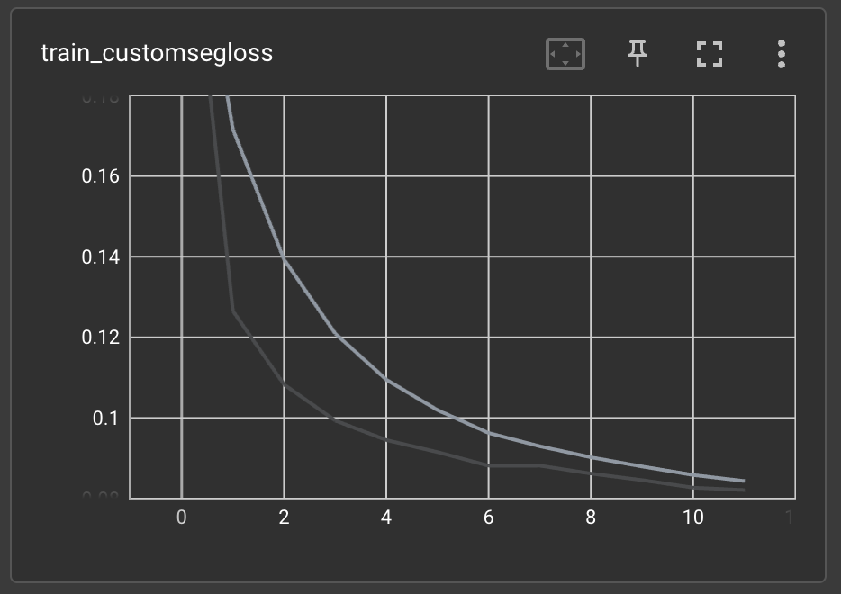
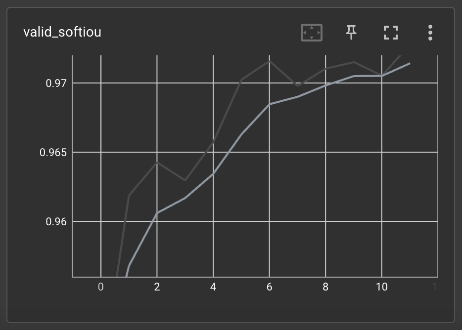
We can also check the validation set's IoU metric's value:
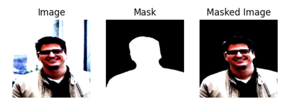
7. Predictions with the trained model
Now that we have a trained model we can use it to make predictions on the test set. First, let's instantiate a test dataset:
test_dataset = AISegmentDataset(data_path=data_path, split='test')
By instantiating the test dataset, all required pre-processing is already handled for us. Let's choose a single sample from the dataset:
image, mask = test_dataset[0]
image, mask = image.unsqueeze(0), mask.unsqueeze(0)
Notice that we have added the batch dimension to the tensors. Next, we set the model to evaluation mode, and obtain the predicted mask. Since our model learned to predict soft masks, we apply a threshold of 0.5 to binarize the mask:
model.eval()

pred = model(image)
pred = torch.gt(pred, 0.5).long()
Finally, let's apply the predicted mask to the image:
masked_image = image*pred
Now let's visualize the image, mask, and masked image to see how our model performed:
figure = plt.figure()
figure.add_subplot(1, 3, 1)
plt.title("Image")
plt.axis("off")
plt.imshow(image.detach().squeeze(0).permute(1, 2, 0))
figure.add_subplot(1, 3, 2)
plt.title("Mask")
plt.axis("off")
plt.imshow(pred.detach().squeeze(0).permute(1, 2, 0), cmap='gray')
figure.add_subplot(1, 3, 3)
plt.title("Masked Image")
plt.axis("off")
plt.imshow(masked_image.detach().squeeze(0).permute(1, 2, 0))
plt.show()