Training a Classification Model and Transfer Learning

In this example we will use SuperGradients to train from scratch a ResNet18 model on the CIFAR10 image classification dataset. We will also fine-tune the same model via transfer learning with weights pre-trained on the ImageNet dataset.

Quick installation

For this example, the only necessary package is super-gradients. Installing super-gradients will also install all dependencies required to run the code in this example.

pip install super-gradients

1. Experiment setup

First, we will initialize the Trainer. It handles: - Model training - Evaluating test data - Making predictions - Saving and managing checkpoints

To initialize it, you need:

• Experiment Name: A unique identifier for your training experiment.
• Checkpoint Root Directory (ckpt_root_dir): The directory where checkpoints, logs, and tensorboards are saved. While optional, if unspecified, it assumes the presence of a 'checkpoints' directory in your project's root.

from super_gradients import Trainer

experiment_name = "resnet18_cifar10_example"
CHECKPOINT_DIR = '/path/to/checkpoints/root/dir'

trainer = Trainer(experiment_name=experiment_name, ckpt_root_dir=CHECKPOINT_DIR)

2. Understanding the Checkpoint Structure

Checkpoints are crucial for progressive training, debugging, and model deployment. SuperGradients organizes them in a structured manner. Here's what the directory hierarchy looks like under your specified ckpt_root_dir:

<ckpt_root_dir>
│
├── <experiment_name>
│   │
│   ├─── <run_dir>
│   │     ├─ ckpt_best.pth                   # Best performance during validation
│   │     ├─ ckpt_latest.pth                 # End of the most recent epoch
│   │     ├─ average_model.pth               # Averaged over specified epochs
│   │     ├─ ckpt_epoch_*.pth                # Checkpoints from specific epochs (like epoch 10, 15, etc.)
│   │     ├─ events.out.tfevents.*           # Tensorflow run artifacts
│   │     └─ log_<timestamp>.txt             # Trainer logs of the specific run
│   │
│   └─── <other_run_dir>
│        └─ ...
│
└─── <other_experiment_name>
    │
    ├─── <run_dir>
    │     └─ ...
    │
    └─── <another_run_dir>
          └─ ...

In this structure:

• ckpt_best.pth: Saved whenever there's an improvement in the specified validation metric.
• ckpt_latest.pth: Updated at the end of every epoch.
• average_model.pth: Averaged checkpoint, created if average_best_models parameter is set to True.

For more information, check out the dedicated page.

2. Dataset and dataloaders

The dataset used in this example is the CIFAR10 image classification dataset.

SuperGradients provides a pool of standard datasets and dataloaders readily available for quick and easy usage. SuperGradients also downloads the datasets when necessary, and gracefully handles the creation of the dataloaders, with a pre-made training recipe specifically tailored for the dataset and model architecture.

Note: The SuperGradients trainer is compatible with PyTorch dataloaders and dataset objects. While it is outside the scope of this example, it is worth remembering that custom dataloaders and datasets can be employed when necessary.

2.A. Default dataloader from SuperGradients

As can be seen in the code snippet below, creating the training and validation dataloaders using SuperGradients' default implementation is as easy as writing two lines of code:

from super_gradients.training import dataloaders

train_dataloader = dataloaders.get(name="cifar10_train", dataset_params={}, dataloader_params={"num_workers": 2})
valid_dataloader = dataloaders.get(name="cifar10_val", dataset_params={}, dataloader_params={"num_workers": 2})

Here, we call the get() function twice, for the training and validation dataloaders. The function's parameters are:

• name - a string representing the name of the desired dataloader, out of a variety of different pre-made dataloaders provided by SuperGradients. In this example, we use the pre-made CIFAR10 training and validation dataloaders.
• dataset_params - a dictionary of dataset-related parameters. Used to override the default parameters defined in the training recipe. Later in this example we will show how this can be used to change the transforms applied to the images.
• dataloader_params - a dictionary of dataloader-related parameters. Used to override the default parameters defined in the training recipe. Here, as an example, we set the number of workers to 2.
• dataset - a torch.utils.data.Dataset object. Used when employing a custom dataset implementation. This parameter cannot be passed together with the name or dataset_params parameters.

We can always print the parameter values of the dataloader and its related dataset:

import pprint

print("Dataloader parameters:")
pprint.pprint(train_dataloader.dataloader_params)

print("Dataset parameters:")
pprint.pprint(train_dataloader.dataset.dataset_params)

Expected output:

Dataloader parameters:
{
    "batch_size": 256,
    "drop_last": False,
    "num_workers": 2,
    "pin_memory": True,
    "shuffle": True
}

Dataset parameters:
{
    "download": True,
    "root": "./data/cifar10",
    "target_transform": None,
    "train": True,
    "transforms": [
        {"RandomCrop": {"size": 32, "padding": 4}},
        "RandomHorizontalFlip",
        "ToTensor",
        {"Normalize": {"mean": [0.4914, 0.4822, 0.4465], "std": [0.2023, 0.1994, 0.201]}},
    ]
}

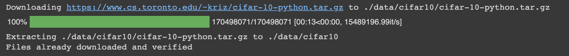
When the get() function is called as above, SuperGradients will attempt to download the CIFAR10 dataset for us. We can expect to see an output as follows:

After the dataloaders are defined, we can iterate them to extract batches of images and their corresponding labels. This is useful for several purposes, such as visualization, verifying tensor shapes, and more. For example, visualization:

from matplotlib import pyplot as plt

def show(images, labels, classes, rows=6, columns=5):
  fig = plt.figure(figsize=(10, 10))

  for i in range(1, columns * rows + 1):
      fig.add_subplot(rows, columns, i)
      plt.imshow(images[i-1].permute(1, 2, 0).clamp(0, 1))
      plt.xticks([])
      plt.yticks([])
      plt.title(f"{classes[labels[i-1]]}")

  plt.show()

images_train, labels_train = next(iter(train_dataloader))
show(images_train, labels_train, classes=train_dataloader.dataset.classes)

Output:

As can be seen, the images are normalized. The normalization process is defined, among other things, as part of the default training recipe SuperGradients uses for the CIFAR10 dataset. As we will see in the following section, SuperGradients makes it a trivial task to override all, or part, of the different dataset and dataloader parameters, allowing for control over the flexibility vs. ease-of-use tradeoff.

For completion of this section, let's print the tensors' shapes:

print(f'Training image tensor shape: {images_train.shape}')
print(f'Training labels tensor shape: {labels_train.shape}')

output:

Training image tensor shape: torch.Size([256, 3, 32, 32])
Training labels tensor shape: torch.Size([256])

As we can see, the default batch size for the training dataloader is 256.

2.B. Override parameters in dataset and dataloaders creation

To showcase the flexibility SuperGradients allows in customizing the different trainer components, we will override the list of transforms that are used in the dataset. To define a list of transformations to apply, we will use torchvision's transforms. This also serves to show the seamless integration SuperGradients allows with different PyTorch components. For the sake of visualization, the only transform we apply is ToTensor(), which simply converts the input images into PyTorch tensors.

from torchvision import transforms as T

transforms_list = [T.ToTensor()]

vis_dataloader = dataloaders.get("cifar10_train",
                                 dataset_params={"transforms": transforms_list},
                                 dataloader_params={"num_workers": 2})

images, labels = next(iter(vis_dataloader))
show(images, labels, classes=train_dataloader.dataset.classes)

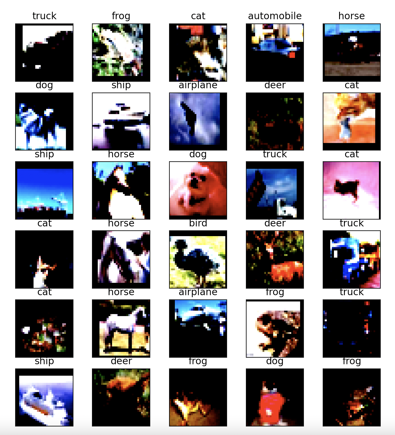
Notice that the only difference in the dataloader's definition is that here, the dataset_params parameter is passed as a dictionary defining the parameters to override. The result of running the above code:

The effect of changing the transforms can be seen in the images - now, without normalization, the objects are more observable in the images.

3. Architecture definition

In this example, we train the model with the ResNet18 architecture.

SuperGradients provides out-of-the-box implementations of many architectures for classification tasks. With just one line of code we can define a model with the chosen architecture. A list of all available architectures can be found here.

from super_gradients.training import models
from super_gradients.common.object_names import Models

model = models.get(model_name=Models.RESNET18, num_classes=10)

Notice that, similar to obtaining a pre-defined dataloader, here we use super_gradients.training.models's get() function. In the above code, two parameters are passed to the function:

• model_name - A string defining the model's architecture name, out of the list of architectures SuperGradients provides.
• num_classes - An integer representing the number of classes the model should learn to predict. Affects the architecture's structure.

Some additional parameters the get() function supports:

• arch_params - A dictionary used to override the default architecture parameters, such as the number of residual blocks.
• checkpoint_path - A string defining the path to an external checkpoint to be loaded. Can be absolute or relative. If provided, will automatically attempt to load the checkpoint.
• pretrained_weights - A string defining the name of a dataset on which the model was pre-trained on, for fine-tuning and transfer learning. The pretrained_weights and checkpoint_path parameters are mutually exclusive.

For more available parameters, refer to the function's docstring.

In this example, we have defined the model with one of SuperGradient's readily available architectures. As was already noted in previous sections, SuperGradients is highly compatible with PyTorch. Defining the model's architecture is not an exception - we can seamlessly use a custom architecture, i.e. a torch.nn.Module object, for maximum flexibility, although it is out of the scope of this example.

4. Training setup

We have defined the trainer, datasets, dataloaders, and model architecture. Before we can start training, we need to define the training parameters. As with the other parameters, SuperGradients provides training parameters optimized for this use-case. For more recommended training parameters you can have a look at our recipes here.

Obtaining the training parameters is as easy as writing a single line of code:

from super_gradients.training import training_hyperparams

training_params =  training_hyperparams.get(config_name="training_hyperparams/cifar10_resnet_train_params")

We notice the repeatability in the code usage - to obtain the training parameters, we again call the get() function. This function accepts two parameters:

• config_name - A string defining the .yaml config filename in the recipes' directory.
• overriding_params - An optional parameter, a dictionary used to override the loaded training parameters.

We can print the training parameters to see the different options:

pprint.pprint("Training parameters:") 
pprint.pprint(training_params)

Output (Training parameters):

{
    '_convert_': 'all',
    'average_best_models': True,
    'batch_accumulate': 1,
    'ckpt_best_name': 'ckpt_best.pth',
    'ckpt_name': 'ckpt_latest.pth',
    'clip_grad_norm': None,
    'cosine_final_lr_ratio': 0.01,
    'criterion_params': {},
    'dataset_statistics': False,
    'ema': False,
    'ema_params': {'decay': 0.9999, 'decay_type': 'exp', 'beta': 15},
    'enable_qat': False,
    'greater_metric_to_watch_is_better': True,
    'initial_lr': 0.1,
    'launch_tensorboard': False,
    'load_opt_params': True,
    'log_installed_packages': True,
    'loss': "CrossEntropyLoss",
    'lr_cooldown_epochs': 0,
    'lr_decay_factor': 0.1,
    'lr_mode': 'StepLRScheduler',
    'lr_schedule_function': None,
    'lr_updates': array([100, 150, 200]),
    'lr_warmup_epochs': 0,
    'lr_warmup_steps': 0,
    'max_epochs': 250,
    'max_train_batches': None,
    'max_valid_batches': None,
    'metric_to_watch': 'Accuracy',
    'mixed_precision': False,
    'optimizer': 'SGD',
    'optimizer_params': {'weight_decay': 0.0001, 'momentum': 0.9},
    'phase_callbacks': [],
    'pre_prediction_callback': None,
    'precise_bn': False,
    'precise_bn_batch_size': None,
    'qat_params': {'start_epoch': 0, 'quant_modules_calib_method': 'percentile', 'per_channel_quant_modules': False, 'calibrate': True, 'calibrated_model_path': None, 'calib_data_loader': None, 'num_calib_batches': 2, 'percentile': 99.99},
    'resume': False,
    'resume_path': None,
    'run_validation_freq': 1,
    'save_ckpt_epoch_list': [],
    'save_model': True,
    'save_tensorboard_to_s3': False,
    'seed': 42,
    'sg_logger': 'base_sg_logger',
    'sg_logger_params': {'tb_files_user_prompt': False, 'launch_tensorboard': False, 'tensorboard_port': None, 'save_checkpoints_remote': False, 'save_tensorboard_remote': False, 'save_logs_remote': False, 'monitor_system': True},
    'silent_mode': False,
    'step_lr_update_freq': None,
    'sync_bn': False,
    'tb_files_user_prompt': False,
    'tensorboard_port': None,
    'train_metrics_list': ['Accuracy', 'Top5'],
    'valid_metrics_list': ['Accuracy', 'Top5'],
    'warmup_initial_lr': None,
    'warmup_mode': 'LinearEpochLRWarmup',
    'zero_weight_decay_on_bias_and_bn': False
}

As can be seen in the above output, there are numerous options to modify the training parameters to affect the training process.

It is also possible to change training parameters after obtaining them, for example:

training_params["max_epochs"] = 15
training_params["sg_logger_params"]["launch_tensorboard"] = True

5. Training, checkpointing, and transfer learning

5.A. Training the model

We are all set to start training our model. Simply plug in the model, training and validation dataloaders, and training parameters into the trainer's train() function:

trainer.train(model=model, 
              training_params=training_params, 
              train_loader=train_dataloader,
              valid_loader=valid_dataloader)

The training progress will be printed to the screen:

[2023-02-01 20:57:27] INFO - sg_trainer_utils.py - TRAINING PARAMETERS:
    - Mode:                         Single GPU
    - Number of GPUs:               1          (4 available on the machine)
    - Dataset size:                 50000      (len(train_set))
    - Batch size per GPU:           256        (batch_size)
    - Batch Accumulate:             1          (batch_accumulate)
    - Total batch size:             256        (num_gpus * batch_size)
    - Effective Batch size:         256        (num_gpus * batch_size * batch_accumulate)
    - Iterations per epoch:         195        (len(train_set) / total_batch_size)
    - Gradient updates per epoch:   195        (len(train_set) / effective_batch_size)

[2023-02-01 20:57:27] INFO - sg_trainer.py - Started training for 15 epochs (0/14)

Train epoch 0: 100%|██████████| 196/196 [00:18<00:00, 10.51it/s, Accuracy=0.262, CrossEntropyLoss=2.37, Top5=0.787, gpu_mem=0.371]
Validation epoch 0: 100%|██████████| 20/20 [00:03<00:00,  6.12it/s]
===========================================================
SUMMARY OF EPOCH 0
├── Training
│   ├── Accuracy = 0.262
│   ├── CrossEntropyLoss = 2.3702
│   └── Top5 = 0.787
└── Validation
    ├── Accuracy = 0.3459
    ├── CrossEntropyLoss = 1.8811
    └── Top5 = 0.871

===========================================================

At the beginning of the training, a summary of the training parameters is printed, where we can see the training mode (CPU/single GPU/distributed training), the number of GPUs used, the training dataset size, and more. The progress of each epoch's training and validation is displayed, along with the tracked metrics (defined as part of the training recipe): accuracy, loss value, top5 error, and GPU memory consumption. At the end of each epoch, a summary of the training and validation metrics is displayed, and in later epochs, a comparison with the previous epochs is provided:

===========================================================
SUMMARY OF EPOCH 15
├── Training
│   ├── Accuracy = 0.7594
│   │   ├── Best until now = 0.7458 (↗ 0.0136)
│   │   └── Epoch N-1      = 0.7458 (↗ 0.0136)
│   ├── CrossEntropyLoss = 0.686
│   │   ├── Best until now = 0.7187 (↘ -0.0327)
│   │   └── Epoch N-1      = 0.7187 (↘ -0.0327)
│   └── Top5 = 0.9867
│       ├── Best until now = 0.9849 (↗ 0.0019)
│       └── Epoch N-1      = 0.9849 (↗ 0.0019)
└── Validation
    ├── Accuracy = 0.7425
    │   ├── Best until now = 0.746  (↘ -0.0035)
    │   └── Epoch N-1      = 0.7306 (↗ 0.0119)
    ├── CrossEntropyLoss = 0.7331
    │   ├── Best until now = 0.7315 (↗ 0.0016)
    │   └── Epoch N-1      = 0.8048 (↘ -0.0717)
    └── Top5 = 0.9831
        ├── Best until now = 0.9838 (↘ -0.0007)
        └── Epoch N-1      = 0.9818 (↗ 0.0013)

===========================================================

At the end of each epoch, the different logs and checkpoints are saved in the path defined by ckpt_root_dir and experiment_name.

In the epoch summary shown above, we can see that the validation accuracy is 73%, which is not very high. To get better insights as to what is happening, we turn to the tensorboard logs.

5.B. Tensorboard logs

To view the experiment's tensorboard logs, type the following command in the terminal from the experiment's path:

tensorboard --logdir='.'

(Alternatively, run the command from anywhere with the experiment's full path).

SuperGradients logs many useful metrics to tensorboard, including CPU and GPU usage, learning rate scheduling, training and validation losses and other metrics, and many more. For the purpose of this example, let us examine the training and validation loss:

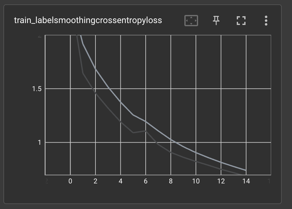
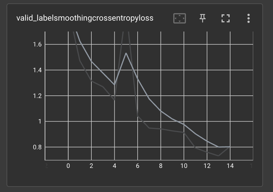
As can be seen in the graphs, the training (and validation) loss did not converge before training ended. This means that training the model for additional epochs will probably improve its performance. Earlier, when modifying the training parameters, we set max_epochs = 15. Let us continue training the model for an additional 10 epochs.

5.C. Continue training from a checkpoint

To continue training from a checkpoint, we utilize the models.get() function's checkpoint_path parameter. The provided checkpoint path includes the checkpoint file we wish to load. In this example, since we want to continue from the last checkpoint, we will load the ckpt_latest.pth checkpoint. Additionally, we want to let the trainer know that we are continuing training and not starting from the first epoch. This is done by setting the resume training parameter to True. Finally, we set the new max_epochs training parameter, and train the model once more.

import os

model = models.get(model_name=Models.RESNET18, 
                   num_classes=10,
                   checkpoint_path=os.path.join(CHECKPOINT_DIR, experiment_name, 'ckpt_latest.pth'))

training_params["resume"] = True
training_params["max_epochs"] = 25

trainer.train(model=model,
              training_params=training_params,
              train_loader=train_dataloader,
              valid_loader=valid_dataloader)

We can see that the training continues for 10 epochs, resuming from epoch 15:

[2023-02-01 21:21:16] INFO - sg_trainer_utils.py - TRAINING PARAMETERS:
    - Mode:                         Single GPU
    - Number of GPUs:               1          (4 available on the machine)
    - Dataset size:                 50000      (len(train_set))
    - Batch size per GPU:           256        (batch_size)
    - Batch Accumulate:             1          (batch_accumulate)
    - Total batch size:             256        (num_gpus * batch_size)
    - Effective Batch size:         256        (num_gpus * batch_size * batch_accumulate)
    - Iterations per epoch:         195        (len(train_set) / total_batch_size)
    - Gradient updates per epoch:   195        (len(train_set) / effective_batch_size)

[2023-02-01 21:21:16] INFO - sg_trainer.py - Started training for 10 epochs (15/24)

Train epoch 15: 100%|██████████| 196/196 [00:18<00:00, 10.52it/s, Accuracy=0.764, CrossEntropyLoss=0.668, Top5=0.987, gpu_mem=0.422]
Validation epoch 15: 100%|██████████| 20/20 [00:03<00:00,  6.10it/s]
===========================================================
SUMMARY OF EPOCH 15
├── Training
│   ├── Accuracy = 0.7644
│   ├── CrossEntropyLoss = 0.6684
│   └── Top5 = 0.9865
└── Validation
    ├── Accuracy = 0.7539
    ├── CrossEntropyLoss = 0.7271
    └── Top5 = 0.9841

===========================================================

Finally, the model stops training after completing 25 epochs:

===========================================================
SUMMARY OF EPOCH 25
├── Training
│   ├── Accuracy = 0.8177
│   │   ├── Best until now = 0.8147 (↗ 0.003)
│   │   └── Epoch N-1      = 0.8147 (↗ 0.003)
│   ├── CrossEntropyLoss = 0.5211
│   │   ├── Best until now = 0.5281 (↘ -0.007)
│   │   └── Epoch N-1      = 0.5281 (↘ -0.007)
│   └── Top5 = 0.9921
│       ├── Best until now = 0.9919 (↗ 0.0002)
│       └── Epoch N-1      = 0.9919 (↗ 0.0002)
└── Validation
    ├── Accuracy = 0.8201
    │   ├── Best until now = 0.7873 (↗ 0.0328)
    │   └── Epoch N-1      = 0.7534 (↗ 0.0667)
    ├── CrossEntropyLoss = 0.525
    │   ├── Best until now = 0.6145 (↘ -0.0895)
    │   └── Epoch N-1      = 0.7517 (↘ -0.2266)
    └── Top5 = 0.9907
        ├── Best until now = 0.9883 (↗ 0.0024)
        └── Epoch N-1      = 0.983  (↗ 0.0077)

===========================================================

We can see that the validation accuracy is now 82%. Much better.

5.C. Transfer learning

So far, we trained a model from scratch. More formally, the model's weights were randomly initialized. For easy tasks and large datasets this is usually sufficient. In other cases, especially when not a lot of data is available for training, we would like to take advantage of knowledge gained from other sources. This is called transfer learning, and it has many forms and variations. In this example we will take a look at the simplest form of transfer learning: fine-tuning a model initialized with pre-trained weights. Specifically, we will initialize our model with weights pre-trained on the ImageNet dataset.

SuperGradients provides a variety of pre-trained weights readily available for fine-tuning different models. To initialize our model with pre-trained weights provided by SuperGradients, only a small change to the existing code is needed:

model = models.get(model_name=Models.RESNET18, num_classes=10, pretrained_weights="imagenet")

In the above code, we provided the pretrained_weights parameter to the models.get() function. This parameter accepts a string representing the name of the dataset that the weights were pre-trained on. Note that this parameter is mutually exclusive with the checkpoint_path parameter.

The rest of the training pipeline is the same as above. For comparison with the previous model, we will train this model for 25 epochs also. Let us look how the model performed:

===========================================================
SUMMARY OF EPOCH 25
├── Training
│   ├── Accuracy = 0.8242
│   │   ├── Best until now = 0.8267 (↘ -0.0025)
│   │   └── Epoch N-1      = 0.8267 (↘ -0.0025)
│   ├── CrossEntropyLoss = 0.5035
│   │   ├── Best until now = 0.4998 (↗ 0.0037)
│   │   └── Epoch N-1      = 0.4998 (↗ 0.0037)
│   └── Top5 = 0.9924
│       ├── Best until now = 0.9917 (↗ 0.0007)
│       └── Epoch N-1      = 0.9917 (↗ 0.0007)
└── Validation
    ├── Accuracy = 0.8377
    │   ├── Best until now = 0.8062 (↗ 0.0315)
    │   └── Epoch N-1      = 0.806  (↗ 0.0317)
    ├── CrossEntropyLoss = 0.4834
    │   ├── Best until now = 0.5731 (↘ -0.0897)
    │   └── Epoch N-1      = 0.5785 (↘ -0.0952)
    └── Top5 = 0.9924
        ├── Best until now = 0.9903 (↗ 0.0021)
        └── Epoch N-1      = 0.9903 (↗ 0.0021)

===========================================================

As we can see, the validation accuracy improved by 1.7% compared to the randomly initialized model. To achieve a greater improvement with pre-trained weights, sometimes careful tuning of the training hyperparameters is required.

6. Predictions with the trained model

Now that we have a trained model with reasonable performance, we can use it to make predictions on new data. First, let's import some packages:

from PIL import Image
import torch
import numpy as np
import requests

Next, we load the model with the trained weights, and put it into evaluation mode. Notice that now we load the ckpt_best.pth checkpoint.

model = models.get(model_name=Models.RESNET18, 
                   num_classes=10,
                   checkpoint_path=os.path.join(CHECKPOINT_DIR, experiment_name, 'ckpt_best.pth'))
model.eval()

We want to test the model on an image of one the classes the model was trained on. As an example, let us test how the model handles an image of a frog, taken from the Aquarium of the Pacific website. The loaded image must undergo the same transformations as the training images for the model to work well:

url = "https://www.aquariumofpacific.org/images/exhibits/Magnificent_Tree_Frog_900.jpg"
image = np.array(Image.open(requests.get(url, stream=True).raw))

transforms = T.Compose([
    T.ToTensor(),
    T.Normalize(mean=(0.4914, 0.4822, 0.4465), std=(0.2023, 0.1994, 0.2010)),
    T.Resize((32, 32))
])

input_tensor = transforms(image).unsqueeze(0).to(next(model.parameters()).device)

Next, to obtain the model's predictions we simply run the following line of code:

predictions = model(input_tensor)

Let's see what the model predicted:

plt.xlabel(train_dataloader.dataset.classes[torch.argmax(predictions)])
plt.imshow(image)
plt.show()

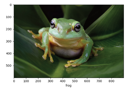
As we can see, the model correctly predicted that the input image is an image of a frog.

7. Complete code

For completion of this example, we provide a complete working code for training, continuing training from a saved checkpoint, and predicting with the trained model. Simply change the CHECKPOINT_DIR variable and run the script:

from super_gradients import Trainer
from super_gradients.training import dataloaders
from super_gradients.training import models
from super_gradients.common.object_names import Models
from super_gradients.training import training_hyperparams
import os
from torchvision import transforms as T
from PIL import Image
import torch
import numpy as np
import requests
import matplotlib.pyplot as plt


def run(experiment_name, CHECKPOINT_DIR):

    # INITIALIZE TRAINER
    trainer = Trainer(experiment_name=experiment_name, ckpt_root_dir=CHECKPOINT_DIR)

    # INITIALIZE DATALOADERS
    train_dataloader = dataloaders.get(name="cifar10_train", dataset_params={}, dataloader_params={"num_workers": 2})
    valid_dataloader = dataloaders.get(name="cifar10_val", dataset_params={}, dataloader_params={"num_workers": 2})

    # DEFINE MODEL
    model = models.get(model_name=Models.RESNET18, num_classes=10)

    # DEFINE TRAINING PARAMETERS
    training_params = training_hyperparams.get(config_name="training_hyperparams/cifar10_resnet_train_params")
    training_params["max_epochs"] = 15

    # TRAIN
    trainer.train(model=model,
                  training_params=training_params,
                  train_loader=train_dataloader,
                  valid_loader=valid_dataloader)

    # LOAD MODEL FROM CHECKPOINT
    model = models.get(model_name=Models.RESNET18,
                       num_classes=10,
                       checkpoint_path=os.path.join(CHECKPOINT_DIR, experiment_name, 'ckpt_latest.pth'))

    # RESUME TRAINING
    training_params["resume"] = True
    training_params["max_epochs"] = 25

    trainer.train(model=model,
                  training_params=training_params,
                  train_loader=train_dataloader,
                  valid_loader=valid_dataloader)

    # LOAD BEST CHECKPOINT
    model = models.get(model_name=Models.RESNET18,
                       num_classes=10,
                       checkpoint_path=os.path.join(CHECKPOINT_DIR, experiment_name, 'ckpt_best.pth'))
    model.eval()

    # PREDICT CLASS FOR TEST IMAGE
    url = "https://www.aquariumofpacific.org/images/exhibits/Magnificent_Tree_Frog_900.jpg"
    image = np.array(Image.open(requests.get(url, stream=True).raw))

    transforms = T.Compose([
        T.ToTensor(),
        T.Normalize(mean=(0.4914, 0.4822, 0.4465), std=(0.2023, 0.1994, 0.2010)),
        T.Resize((32, 32))
    ])

    input_tensor = transforms(image).unsqueeze(0).to(next(model.parameters()).device)

    predictions = model(input_tensor)

    plt.xlabel(train_dataloader.dataset.classes[torch.argmax(predictions)])
    plt.imshow(image)
    plt.show()


if __name__ == '__main__':

    experiment_name = "resnet18_cifar10_example"
    CHECKPOINT_DIR = '/path/to/checkpoints/root/dir'

    run(experiment_name, CHECKPOINT_DIR)